The concept of integrating machine learning into crime datasets is not new. Several researchers have dedicated efforts to apply different models to different segments of the data, including the specific aspect of crime resolution.
This diversity in approaches reflects the complexity and many-sided nature of crime data, where predictive models can vary in effectiveness based on the particular characteristics of the data, such as geographical variables, types of crimes, and temporal factors. In addition, addressing the challenge of racism in machine learning models applied to crime data is both vital and commendable. By focusing on the ethical dimensions and consciously removing racial and ethnic characteristics from our models, we as a society are taking a significant step towards ensuring fairness and preventing bias in predictive models.
Having said that, my primary goal was not to create a perfect model(with the highest accuracy) but rather to develop a fair model. Such effort is essential in advancing the responsible use of AI in societal applications, where the consequences of biased algorithms can be profound.
The data
The dataset utilized in this project originates from the Murder Accountability Project, a comprehensive database of homicide records in the United States, sourced from Kaggle. It includes over 600,000 cases recorded between 1980 and 2014. This data is among the most detailed compilations existing today, featuring in-depth reports from the FBI’s Supplementary Homicide Report, which has been ongoing since 1976. It also includes information from over 22,000 homicide cases not officially reported to the Justice Department, obtained through the Freedom of Information Act.
Compiled and made publicly accessible by the Murder Accountability Project under the guidance of Thomas Hargrove, these records aim to enhance transparency concerning homicide rates and the efficacy of justice systems in the U.S. The initiative emphasizes the critical role of open data in addressing societal issues and promoting accountability within the realm of criminal justice.
The table offers a detailed breakdown of each case, documenting elements such as:
- Record ID: The identifier for each crime.
- Agency Code: The code representing the involved agency.
- Agency Name: The name of the agency.
- Agency Type: The type of agency reporting the crime.
- City: The city where the crime occurred.
- State: The state where the crime occurred.
- Year: The year the crime was committed.
- Month: The month the crime was committed.
- Incident: The number of related incidents.
- Crime Type: Specifies whether the crime was Murder or Manslaughter/Manslaughter by Negligence.
- Crime Solved: Indicates whether the crime was solved.
- Victim Sex: Gender of the victim.
- Victim Age: Age of the victim.
- Victim Race: Race of the victim.
- Victim Ethnicity: Ethnicity of the victim.
- Perpetrator Sex: Gender of the perpetrator.
- Perpetrator Age: Age of the perpetrator.
- Perpetrator Race: Race of the perpetrator.
- Perpetrator Ethnicity: Ethnicity of the perpetrator.
- Relationship: The relationship between the victim and the perpetrator.
- Weapon: The weapon used in the crime.
- Victim Count: The number of victims involved.
- Perpetrator Count: The number of perpetrators involved.
- Record Source: The source from which the data was obtained.
Explanatory Data Analysis
Exploratory Data Analysis, known as EDA, is a phase in the data analysis process that involves summarizing the main characteristics of a dataset, often visualizing them in a way that is easily accessible and understandable. The primary goal of EDA is to examine the data for distribution, outliers, and anomalies to inform subsequent analysis stages and ensure valid model assumptions.
This process helps in uncovering underlying patterns, spotting anomalies, testing a hypothesis, or checking assumptions with the help of summary statistics and graphical representations.
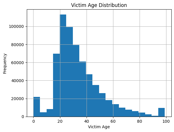
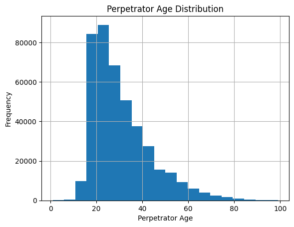
To start, I examine the age distributions of both victims and perpetrators in crime incidents. The histograms reveal distinct age-related patterns, suggesting that certain age groups are more frequently involved either as victims or perpetrators.
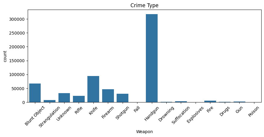
Delving deeper into the types of crimes committed with various weapons, the data shows that handguns are predominantly used in murders and assaults. This insight supports the hypothesis that certain weapons are preferred in specific types of crimes, which could guide law enforcement in focusing their efforts on specific weapon regulations and controls.
To check the monotonic relationships between numerical variables, I calculated The Spearman correlation coefficient. A significant positive correlation (0.76) suggests that as the age of the perpetrator increases, the likelihood of solving the crime increases.
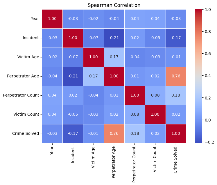
There is a moderate positive correlation (0.17) between these variables, implying that crimes involving older victims also tend to involve older perpetrators.
A modest correlation (0.18) indicates that incidents involving more perpetrators have a slightly higher probability of being solved. The correlation coefficient (0.02) is low, suggesting a weak relationship between the number of victims and the resolution of a crime.
To determine the strength of association between categorical variables in the crime dataset, I performed a Chi-Square analysis.
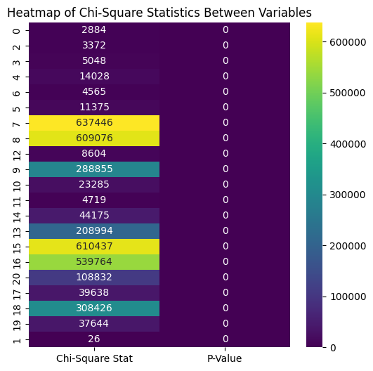
The strongest association observed is between “Perpetrator Sex” and “Crime Solved.” This suggests that the gender of the perpetrator might influence the likelihood of crime resolution. There are strong associations between “Perpetrator Sex” and “Perpetrator Race,” as well as between “Victim Sex” and these perpetrator characteristics.
“Crime Type” shows notable correlations with “Relationship” and “Weapon,” which underscores the interconnectedness of the nature of the crime with both the relationship to the victim and the means used to commit the crime. Although the relationship between “Crime Type” and “Victim Sex” shows a weaker Chi-square statistic relative to others, the very low P-value confirms its statistical significance.
Machine Learning Models for solving a crime - Logistic Regression, Decision Tree, XGBoost and Random Forest.
When applying machine learning to the problem of solving crime, several models stand out for their effectiveness and unique capabilities.
Each of these models can contribute differently to solving crimes. Logistic regression could be used for initial screening to estimate the probability of crime occurrence. Decision trees and random forests are excellent at classification tasks such as identifying the type of crime based on various inputs. XGBoost, being a powerful algorithm that handles various types of data effectively, can be used for more complex tasks like predicting crime hotspots and understanding the factors that influence crime rates.
The base model - Logistic Regression
Logistic regression, as a simple and interpretable model, provides a valuable benchmark against which more complex models can be compared. By measuring its performance, one can establish a baseline for what can be achieved without delving into more computationally expensive or complex algorithms.
Data Preprocessing
In preparation for analysis, the dataset underwent a series of preprocessing steps:
- Binary Encoding: The ‘Crime Solved’ variable was encoded into binary format, with ‘Yes’ mapped to 1 (solved) and ‘No’ to 0 (not solved).
- Feature Selection: Unnecessary columns such as agency codes and personal identifiers were removed to focus on relevant variables like “Weapon”, “Relationship”, “Incident”,“Crime Type”, “Victim Count” and “Perpetrator Count”.
- Pipeline Implementation: Separate preprocessing pipelines were established for numerical and categorical data, incorporating imputation of missing values, standardization, and one-hot encoding.
Model Implementation and Evaluation
The base model for this analysis, chosen for its simplicity and interpretability:
- Model Training: A logistic regression model was integrated within a pipeline that included the preprocessing steps and was trained using a stratified sample of the data.
- Model Tuning: Hyperparameter tuning was conducted using GridSearchCV to optimize the regularization strength of the logistic regression algorithm.
- Evaluation Metrics: The model’s performance was assessed through accuracy, precision, recall, and F1-score, providing a comprehensive view of its predictive capabilities.
Findings and Insights
The base model provided a solid foundation for understanding the impact of various features on crime-solving outcomes:
- Feature Importance: Analysis of model coefficients revealed significant predictors such as ‘Weapon’ and ‘Relationship’, highlighting their influence on whether a crime gets solved.
- Model Performance: The model achieved an initial accuracy score, serving as a benchmark for subsequent model comparisons.
Below is the complete code:
import pandas as pd
from sklearn.model_selection import train_test_split, StratifiedShuffleSplit, GridSearchCV
from sklearn.compose import ColumnTransformer
from sklearn.pipeline import Pipeline
from sklearn.impute import SimpleImputer
from sklearn.preprocessing import StandardScaler, OneHotEncoder
from sklearn.linear_model import LogisticRegression
from sklearn.metrics import classification_report, accuracy_score

# Load the dataset
crime = pd.read_csv('database.csv')  # Adjust the path as necessary

# Assume 'Crime Solved' is binary and needs to be encoded
crime['Crime Solved'] = crime['Crime Solved'].map({'Yes': 1, 'No': 0})

# Drop columns that are not useful
#crime = crime.drop(["Record ID", "Agency Code", "Agency Name", "Agency Type", "Record Source", "Year", "Month", "Victim Count", "Perpetrator Count", "Victim Sex", "Victim Age", "Victim Race", "Victim Ethnicity", "Perpetrator Sex", "Perpetrator Age", "Perpetrator Race", "Perpetrator Ethnicity", "Victim Count"], axis=1)
crime=crime[["Weapon", "Relationship", "Crime Solved", "Incident", "Crime Type", "Victim Count", "Perpetrator Count"]]
print(crime.columns)

# Define features and target variable
X = crime.drop('Crime Solved', axis=1)
y = crime['Crime Solved']

# Stratified sampling to maintain class distribution
sss = StratifiedShuffleSplit(n_splits=1, test_size=0.05, random_state=42)  # Using 5% of the data
for train_index, test_index in sss.split(X, y):
    X_sample, y_sample = X.iloc[test_index], y.iloc[test_index]

# Split the sampled data into training and test sets
X_train, X_test, y_train, y_test = train_test_split(X_sample, y_sample, test_size=0.2, random_state=123)

# Identifying numerical and categorical columns
numerical_cols = X_train.select_dtypes(include=['int64', 'float64']).columns
categorical_cols = X_train.select_dtypes(include=['object']).columns

# Creating preprocessing pipelines for numerical and categorical features
numerical_pipeline = Pipeline([
    ('imputer', SimpleImputer(strategy='median')),
    ('scaler', StandardScaler())
])

categorical_pipeline = Pipeline([
    ('imputer', SimpleImputer(strategy='most_frequent')),
    ('encoder', OneHotEncoder(handle_unknown='ignore'))
])

# Combine preprocessing steps
preprocessor = ColumnTransformer([
    ('num', numerical_pipeline, numerical_cols),
    ('cat', categorical_pipeline, categorical_cols)
])

# Creating the full pipeline with logistic regression
pipeline = Pipeline([
    ('preprocessor', preprocessor),
    ('classifier', LogisticRegression(random_state=42, solver='liblinear'))
])

# Fit the model
pipeline.fit(X_train, y_train)

# Predict and evaluate the model
y_predicted = pipeline.predict(X_test)
print("Classification Report: \n", classification_report(y_test, y_predicted))
print("Accuracy: ", accuracy_score(y_test, y_predicted))

# Optional: Setting up GridSearchCV for hyperparameter tuning
param_grid = {
    'classifier__C': [0.1, 1.0, 10]
}
grid_search = GridSearchCV(pipeline, param_grid, cv=5, scoring='accuracy')
grid_search.fit(X_train, y_train)
print("Best parameters:", grid_search.best_params_)
print("Best cross-validated accuracy:", grid_search.best_score_)

import matplotlib.pyplot as plt
import numpy as np

# Assuming Logistic Regression is the classifier in the last step of the pipeline
feature_names = numerical_cols.tolist() + list(pipeline.named_steps['preprocessor'].transformers_[1][1].named_steps['encoder'].get_feature_names_out(categorical_cols))
coefficients = pipeline.named_steps['classifier'].coef_[0]

# Combine feature names and their coefficients
feature_importance = list(zip(feature_names, coefficients))
feature_importance.sort(key=lambda x: abs(x[1]), reverse=True)  # Sort by absolute value of coefficients

# Splitting names and values for plotting
features, importance = zip(*feature_importance)

# Plotting
plt.figure(figsize=(10, 8))
plt.barh(features[:20], importance[:20], color='dodgerblue')  # Only display top 20 features
plt.xlabel('Coefficient Magnitude')
plt.ylabel('Feature')
plt.title('Top 20 Feature Importances in Logistic Regression Model')
plt.gca().invert_yaxis()  # Invert the y-axis to have the most important at the top
plt.show()
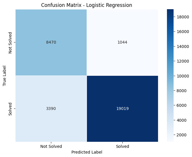
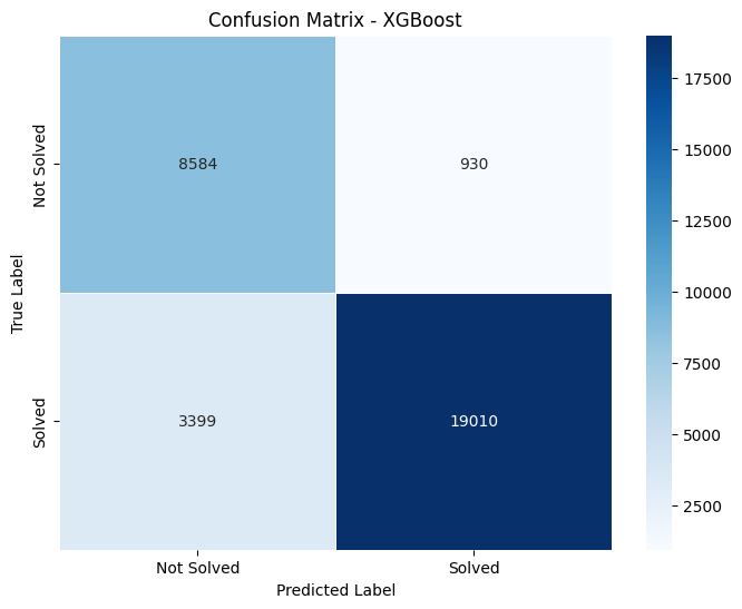
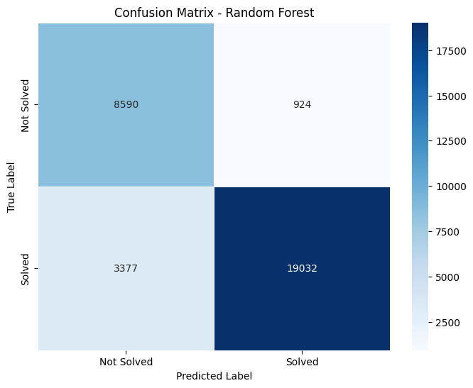
Combined Confusion matrix
Confusion matrices are a performance measurement for machine learning classification problems. Here are the details extracted from the matrices:

Confusion Matrix Details
- Decision Tree: True Negative (TN): 8588 False Positive (FP): 926 False Negative (FN): 3910 True Positive (TP): 18959
- Logistic Regression: TN: 8470 FP: 1044 FN: 3390 TP: 19018
- XGBoost: TN: 8584 FP: 930 FN: 3399 TP: 19501
- Random Forest: TN: 8580 FP: 934 FN: 3377 TP: 19023
True Positives (TP) represent the number of correct predictions that an instance is positive. True Negatives (TN) represent the number of correct predictions that an instance is negative. False Positives (FP), often considered a type error, indicate the number incorrectly identified as positive. False Negatives (FN), another type of error, indicate the number incorrectly identified as negative.
As we compare the given metrics, it is cleran that XGBoost has the highest number of True Positives (19501), suggesting it is the best model among the four for correctly predicting positive cases.Decision Tree and Random Forest show similar performance in terms of True Negatives, but Random Forest has slightly fewer False Negatives, suggesting slightly better sensitivity than the Decision Tree.
Logistic Regression, while having the highest number of True Negatives, also has a slightly higher number of False Positives compared to other models, indicating it might be less precise in predicting positive cases.
From my analysis, XGBoost appears to be the most effective model for this specific dataset in terms of overall predictive accuracy, particularly in correctly identifying positive cases. Logistic Regression, while robust, may require adjustments to reduce the number of False Positives.
Each model has strengths and weaknesses, and the choice of model could depend on the specific requirements of the application, such as prioritizing the reduction of False Positives or False Negatives.
All in all
Now it is time to compare all four models in terms of the most important model measurements.
Below, you can see a plot that has the following metrics:
- Accuracy: Compares the accuracy of Logistic Regression, Random Forest, XGBoost, and Decision Tree.
- Precision: Compares the precision of the same models.
- Recall: Compares the recall of the same models.
- F1-Score: Compares the F1-score of the same models.
- AUC (Area Under the Curve): Compares the AUC of the same models.
- Best Cross-Validated Accuracy: Compares the best cross-validated accuracy of the same models.
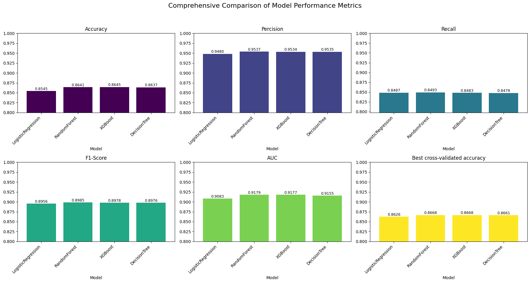
The extensive calculations show the following:
Accuracy:
- Logistic Regression: ~0.8545
- Random Forest: ~0.8641
- XGBoost: ~0.8645
- Decision Tree: ~0.8637
Precision:
- Logistic Regression: ~0.9480
- Random Forest: ~0.9537
- XGBoost: ~0.9534
- Decision Tree: ~0.9535
Recall:
- Logistic Regression: ~0.8487
- Random Forest: ~0.8493
- XGBoost: ~0.8483
- Decision Tree: ~0.8478
F1-Score:
- Logistic Regression: ~0.8956
- Random Forest: ~0.8985
- XGBoost: ~0.8978
- Decision Tree: ~0.8976
AUC:
- Logistic Regression: ~0.9083
- Random Forest: ~0.9179
- XGBoost: ~0.9177
- Decision Tree: ~0.9155
Best Cross-Validated Accuracy:
- Logistic Regression: ~0.8626
- Random Forest: ~0.8668
- XGBoost: ~0.8668
- Decision Tree: ~0.8661
Random Forest and XGBoost perform similarly across all metrics, consistently showing high values especially in precision, F1-score, and AUC. Decision Tree has performance metrics very close to XGBoost and Random Forest, indicating it is also a robust model, although slightly lower in some aspects like recall and best cross-validated accuracy. Logistic Regression shows the lowest accuracy and best cross-validated accuracy among the models, but still performs reasonably well, especially in precision and AUC. For applications requiring high precision, the Decision Tree and XGBoost are preferable, while Random Forest might be chosen for slightly better overall balance in performance.
For the complete code, notebooks, and plots used in these analyses, please visit my repository at Github.